Creating a Quantitative Trading Strategy Based on Sentiment Data
TL;DR - The research workflow of a quantitative trading project.
December 30, 2017
Over this past semester, I developed a quantitative trading strategy that used sentiment data from news sites and social media. These notes cover my research workflow for strategy identification and backtesting. I chose to use the Quantopian platform because it gave access to rich datasets, an easy to use IDE, and a backtesting environment that allowed me to take code written in my research notebooks and directly use it in the trading algorithm.
Strategy Identification and Backtesting Workflow
Data
I used the Sentdex dataset, which "assesses the sentiment of companies by pulling from over 20 sources such as Wall Street Journal, CNBC, Forbes, Business Insider, and Yahoo Finance." The dataset's primary factor was sentiment signal, which is a standalone sentiment score from -3 to 6 for equities. I also used Quantopian's US Equity Pricing dataset which can be filtered to your strategy's specifications.
"Sentiment analysis refers to the use of natural language processing, text analysis, computational linguistics, and biometrics to systematically identify, extract, quantify, and study affective states and subjective information."
The trading strategy's performance is reliant upon the chosen equity universe. I chose to use the Q1500US as my base, which is made up of 1500 stocks that are suitable for trading. It throws out hard-to-trade equities like non-primary shares, stocks, with missing data, etc. Only the top 1500 stocks based on 200-day Average Dollar Volume (which is a measure of liquidity, aka h) are kept.
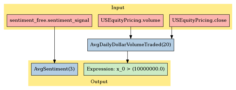
To take the data from the Sentdex and US Equity Pricing datasets, I used Pipeline, Quantopian's trading infrastructure implementation to dynamically select equities from the base universe. Optimally, it's meant to be used in both the research notebooks as well as the trading algorithm. To filter out low liquidity stocks in the Q1500US, an average daily dollar volume traded filter was applied.
      class AvgDailyDollarVolumeTraded(CustomFactor):
          window_length = 20
          inputs = [USEquityPricing.close, USEquityPricing.volume]
          def compute(self, today, assets, out, close_price, volume):
              out[:] = np.mean(close_price * volume, axis=0)
Alpha Discovery
After the Pipeline was set up, the goal of the next stage, alpha discovery, was to evaluate a range of alpha factors and their respective predictive abilities for stock prices.
"Alpha factors express a predictive relationship between some given set of information and future returns."
I chose 8 factors to test: bullish intensity and bearish intensity from the PsychSignal dataset, sentiment sigal, and a simple moving average of the sentiment signal over window lengths of 3, 10, 20, 30, 50, and 80, which were taken from the Sentdex dataset. A moving average is commonly used with financial data "to smooth out short-term fluctuations and highlight longer-term trends or cycles." My hypothesis was that after an event occurs that triggers some change in equity price, overall sentiment, in the form of news articles and social media posts lag behind shortly after. I configured each factor in Pipeline and used Alphalens, a Python package used for performance analysis of alpha factors, to generate a tearsheet of each which contains relavent statistics and plots.
The simple moving average of sentiment signal over 3 days (average sentiment signal) had the best performance out of the 8 alpha factors tested. AvgSentiment implementation:
      class AvgSentiment(CustomFactor):
          def compute(self, today, assets, out, impact):
              np.mean(impact, axis=0, out=out)
AvgSentiment used the the input sentiment_signal and averaged it over a particular window length.
      window_length =3
      pipe = Pipeline()
      dollar_volume = AvgDailyDollarVolumeTraded()
      pipe.add(Sector(), 'Sector')

      # Add our AvgSentiment factor to the pipeline using a 3 day moving average
      pipe.add(AvgSentiment(inputs=[sentiment_free.sentiment_signal], window_length=window_length), "avg_sentiment")

      # Screen out low liquidity securities.
      pipe.set_screen((dollar_volume > 10**7))
      start_timer = time()
      results = run_pipeline(pipe, '2015-01-01', '2016-01-01')
      end_timer = time()

      # Times how long the pipeline takes to run.
      print("Time to run pipeline %.2f secs" % (end_timer - start_timer))
      adjusted_dataset = results.interpolate()
Looking at results,
results.head()
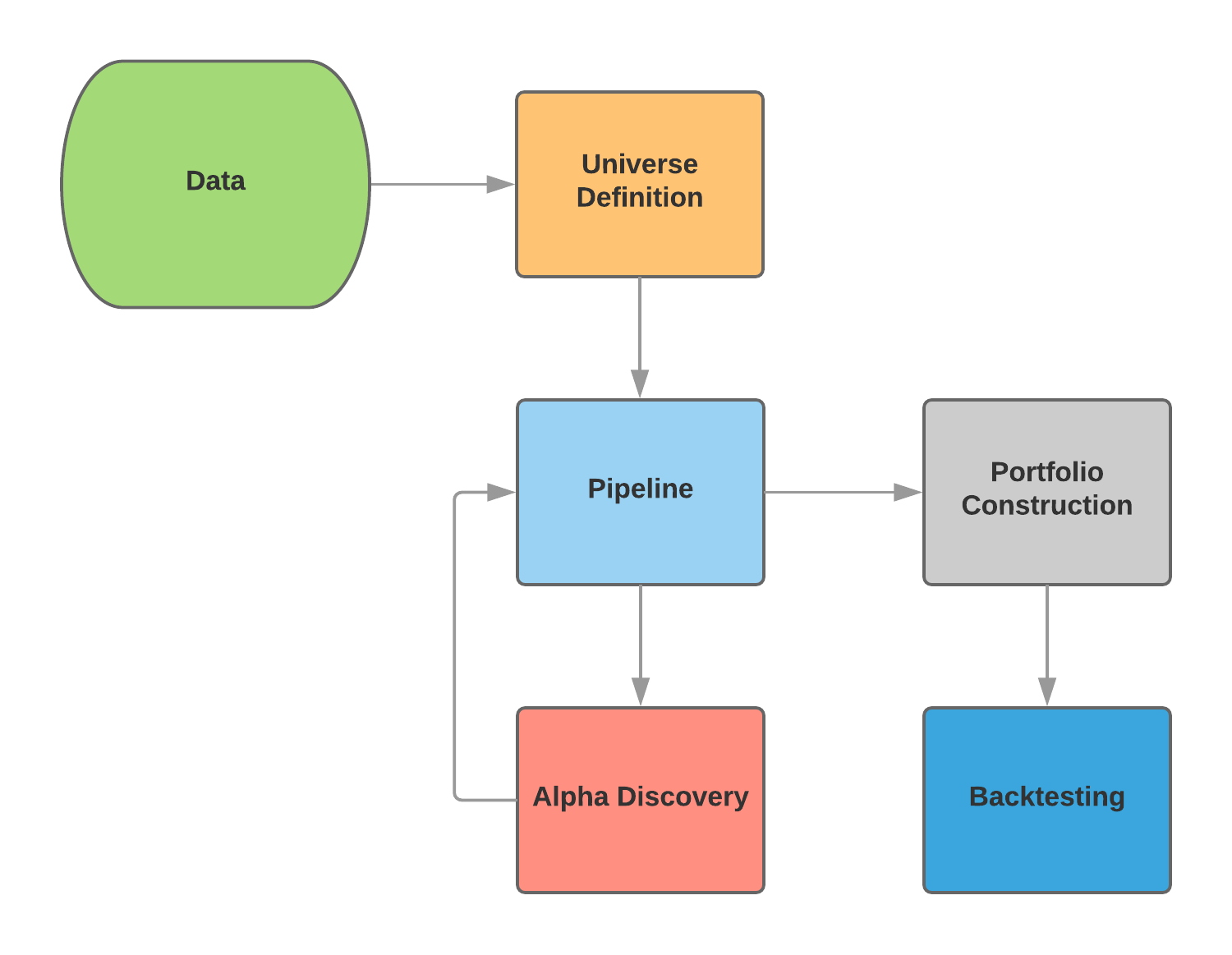
many of the equities were listed multiple times and also there were many NaN values. To adjust for NaN values, Pandas' interpolate() function was used, which constructed new data points within the range of the existing ones by taking the mean of the data above and below it when ordered. Graphically, the Pipeline looked like the following:
Pipeline Representation
To deal with repeated equities in results:
      #Asset list extraction.
      avgsent_factor = adjusted_dataset["avg_sentiment"]
      sectors = adjusted_dataset['Sector']
      asset_list = adjusted_dataset.index.levels[1].unique()
      prices = get_pricing(asset_list, start_date='2015-01-01', end_date='2016-01-01', fields='price')
The asset_list contained all unique equities from the adjusted dataset. The avgsent_factor and sectors were their respective columns, and prices was a Pandas DataFrame of the prices for the equities in asset_list. Here is how the tearsheet of relavent statistics for your alpha factor was generated through the Alphalens package:
      avgsent_factor_data = al.utils.get_clean_factor_and_forward_returns(
                                                                factor=avgsent_factor,
                                                                prices=prices,
                                                                groupby=sectors,
                                                                quantiles=2,
                                                                groupby_labels=MORNINGSTAR_SECTOR_CODES,
                                                                periods=(1, 5, 10))
      avgsent_factor_data.head()
      al.tears.create_full_tear_sheet(avgsent_factor_data)
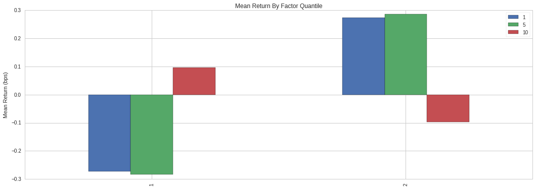
Mean Returns by Factor Quantile
The plot above described the optimal window length for which the alpha factor, average sentiment, was most predictive. It was broken down by 1, 5, and 10 days. The visualization showed that average sentiment operated best as a short-term predictor, and that 1 and 5 days were very similar, with a steep drop off by 10 days. Quantile 1 and 2 represented the short and long positions, respectively. This graph confirms that a window length of 3 days works well to predict stock price because it fits nicely between 1 and 5 days on the plot and it has the largest absolute value for both the short and long quantiles.
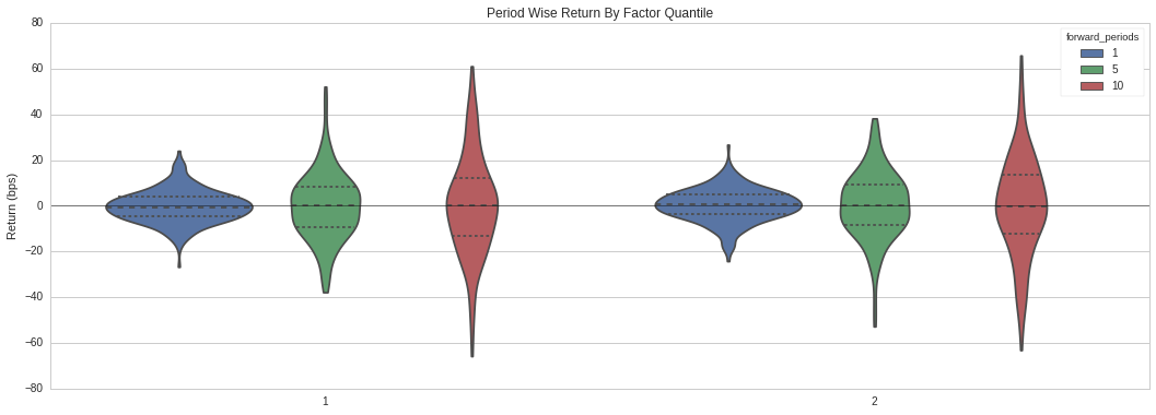
Period Wise Return by Factor Quantile
The violin plot of our timeseries of quantile 1 and 2 (short and long positions, respectively) shows that a 1 day period had the highest density of returns and values relatively close to the mean.
Strategy
I worked with a long-short equity strategy, which involved maintaining a long position on equities that were supposed to increase in price and maintaining a short position on equities that were supposed to decrease in price. The equities were then ranked by the average sentiment factor. If the average sentiment value associated with the corresponding equity was greater than 0, it was put in the long basket and if it was less than 0, it was put in the short basket. The strategy then ordered all the equities in the long and short baskets one hour after the market opened each day, and was rebalanced every day. This strategy worked best with a very high starting capital and is market neutral so it could perform well in any economic climate. The goal was to minimize exposure to the market, while maximizing returns.
Backtesting
The last step was backtesting the trading algorithm. The custom factors AverageSentiment and AverageDailyDollarVolumeTraded can be used directly in our algorithm, as well as the Pipeline created in the research notebook. In the Quantopian API, there were 3 functions that were necessary for the trading algorithm to work: before trading start, handle_data, and rebalance.
Before_trading_start was an optional method called once a day, before the market opened. It was used to deal with the NaN values, declare long and short positions, and rank the equities based on the average sentiment factor. Every day, this function was called and the positions were updated. Handle_data was called every minute to get individual prices and windows of prices for one or more assets. An algorithm's leverage, number of portfolio positions, and the number of open orders can be adjusted. Rebalance was called every day 1 hour after the market opened and placed the equity orders. Implementation for the full trading algorithm:
      from quantopian.algorithm import attach_pipeline, pipeline_output
      from quantopian.pipeline import Pipeline
      from quantopian.pipeline.data.builtin import USEquityPricing
      from quantopian.pipeline.factors import CustomFactor
      from quantopian.pipeline.data.sentdex import sentiment_free as sentdex
      import pandas as pd
      import numpy as np

      class AverageSentiment(CustomFactor):
          def compute(self, today, assets, out, impact):
              np.mean(impact, axis=0, out=out)

      class AverageDailyDollarVolumeTraded(CustomFactor):
          window_length = 20
          inputs = [USEquityPricing.close, USEquityPricing.volume]
          def compute(self, today, assets, out, close_price, volume):
              out[:] = np.mean(close_price * volume, axis=0)

      def initialize(context):
          window_length = 3
          pipe = Pipeline()
          pipe = attach_pipeline(pipe, name='Sentiment_Pipe')
          dollar_volume = AverageDailyDollarVolumeTraded()
          filter = (dollar_volume > 10**7)

          pipe.add(AverageSentiment(inputs=[sentdex.sentiment_signal],
                                window_length=window_length), 'Average_Sentiment')
          pipe.set_screen(filter)
          context.longs = None
          context.shorts = None

          schedule_function(rebalance, date_rules.every_day(), time_rules.market_open(hours=1))
          set_commission(commission.PerShare(cost=0, min_trade_cost=0))
          set_slippage(slippage.FixedSlippage(spread=0))

      def before_trading_start(context, data):
          results = pipeline_output('Sentiment_Pipe').dropna()

          longs = results[results['Average_Sentiment'] > 0]
          shorts = results[results['Average_Sentiment'] < 0]

          long_ranks = longs['Average_Sentiment'].rank().order()
          short_ranks = shorts['Average_Sentiment'].rank().order()

          num_stocks = min([25, len(long_ranks.index), len(short_ranks.index)])

          context.longs = long_ranks.head(num_stocks)
          context.shorts = short_ranks.tail(num_stocks)

          update_universe(context.longs.index | context.shorts.index)

      def handle_data(context, data):
          #num_positions = [pos for pos in context.portfolio.positions
          #                 if context.portfolio.positions[pos].amount != 0]
          record(lever=context.account.leverage,
                 exposure=context.account.net_leverage,
                 num_pos=len(context.portfolio.positions),
                 oo=len(get_open_orders()))


      def rebalance(context, data):

          for secuhttps://www.quantopian.com/algorithmsrity in context.shorts.index:
              if get_open_orders(security):
                  continue
              if security in data:
                  order_target_percent(security, -1.0 / len(context.shorts))

          for security in context.longs.index:
              if get_open_orders(security):
                  continue
              if security in data:
                  order_target_percent(security, 1.0 / len(context.longs))

          for security in context.portfolio.positions:
              if get_open_orders(security):
                  continue
              if security in data:
                  if security not in (context.longs.index | context.shorts.index):
                          order_target_percent(security, 0)
A full backtest was completed from 6/3/2014 to 10/25/2017 because the Sentdex dataset only goes back so far. When it finished, the backtest was analyzed with Alphalens in the research notebook (string is the backtest code).
      bt = get_backtest('5a1971b0a7a94b4499ca39ff')
      bt.create_full_tear_sheet()
The plot below showed the cummulative returns of the strategy versus the Standard and Poor's 500 from June 3, 2014 to October 25, 2017. The first 2 years, the strategy outperformed the benchmark and ended up matching the benchmark's performance by the end of the backtest.
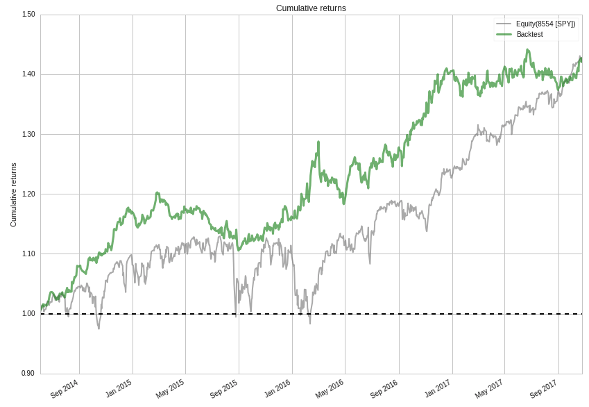
Cummulative Returns of Trading Strategy vs. SPY
Cummulative returns don't give the full story of a trading algorithm's performance. The plot below showed the rolling volatility (6 months) of the trading algorithm versus the SPY benchmark, as well as the average volatility of trading algorithm. The trading strategy had a lower volatility than the benchmark and greater returns up to the last few months of 2017.
"Volatility is a statistical measure of the disperion of returns for a given security or market index. Commonly, the higher the volatility, the riskier the security."
If you have any questions, feel free to send me an email.